[说明] : 以下是高度可复用代码。在此做个总结和公开。
0. 预热,一些经典的设置
pd.set_option('display.float_format',lambda x: '%.2f'%x)
pd.set_option('display.expand_frame_repr',False)
#显示所有列
pd.set_option('display.max_columns', None)
#显示所有行
#pd.set_option('display.max_rows', None)
pd.set_eng_float_format(accuracy=1, use_eng_prefix=True)--一位小数,结尾用k、M表示
1. EDA
单变量分布
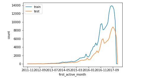
- 校验train和test上的特征分布是否相似(图像)
# 以features为例分析训练集与测试集的差异
features = ['first_active_month','feature_1','feature_2','feature_3']
train_count = train.shape[0]
test_count = test.shape[0]
for feature in features:  # 对每一个特征进行枚举
    train[feature].value_counts().sort_index().plot()
    test[feature].value_counts().sort_index().plot()
    plt.xlabel(feature)
    plt.legend(['train','test'])
    plt.ylabel('count')
    plt.show()
如图所示:
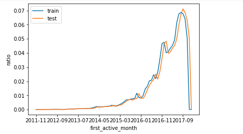
- 校验train和test上的特征分布是否相似(数据)
features = ['first_active_month','feature_1','feature_2','feature_3']
train_count = train.shape[0]
test_count = test.shape[0]
for feature in features:
    (train[feature].value_counts().sort_index()/train_count).plot()  # 得到的是比率
    (test[feature].value_counts().sort_index()/test_count).plot()
    plt.legend(['train','test'])
    plt.xlabel(feature)
    plt.ylabel('ratio')
    plt.show()
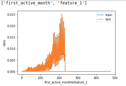
多变量联合分布
- 离散状态下,使用特征拼接 。查看拼接后特征的分布
def combine_feature(df):
    cols = df.columns
    feature1 = df[cols[0]].astype(str).values.tolist()
    feature2 = df[cols[1]].astype(str).values.tolist()
    return pd.Series([feature1[i]+'&'+feature2[i] for i in range(df.shape[0])])

n = len(features)  # 探究f的长度
for i in range(n-1):
    for j in range(i+1, n):
        cols = [features[i], features[j]]  # 拼接
        print(cols)
        train_dis = combine_feature(train[cols]).value_counts().sort_index()/train_count
        test_dis = combine_feature(test[cols]).value_counts().sort_index()/test_count
        index_dis = pd.Series(train_dis.index.tolist() + test_dis.index.tolist()).drop_duplicates().sort_values()
        (index_dis.map(train_dis).fillna(0)).plot()
        (index_dis.map(test_dis).fillna(0)).plot()
        plt.legend(['train','test'])
        plt.xlabel('&'.join(cols))
        plt.ylabel('ratio')
        plt.show()
离散字段的数量分布
# 简单看下每个离散字段Top10的数量分布
for col in category_cols[1:]:
    merchant[col].astype(str).value_counts()[:10].sort_index().plot.bar()
    plt.show()
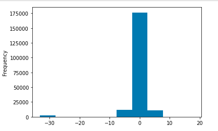
目标值的观察
- 连续
train['target'].plot.hist()
plt.show()
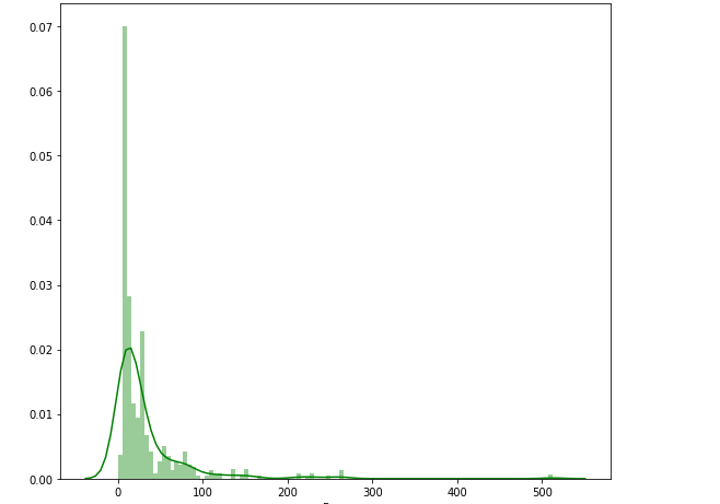
带有线条的直方图
plt.figure(figsize=(9,8))
sns.distplot(train['Fare'] , color = 'g'  , bins = 100 , hist_kws = {'alpha' : 0.4})
热力图的绘制
f , ax  = plt.subplots(figsize = (30,30))
sns.heatmap(corrmat , vmax = 0.8 , square = True , cmap="gist_rainbow")
rainbow 是我选择的比较不错的配色,集美观和实用于一体。明显区别出来相关特征,简而言之,heatmap里面的绿色标记是不需要注意的。还有大量其他配色,我列在下面。
使用cmap可以改变图的颜色,蓝色、粉红色·和红色等,cmap可以选择:
Accent, Accent_r, Blues, Blues_r, BrBG, BrBG_r, BuGn, BuGn_r, BuPu, BuPu_r, CMRmap, CMRmap_r, Dark2, Dark2_r, GnBu, GnBu_r, Greens, Greens_r, Greys, Greys_r, OrRd, OrRd_r, Oranges, Oranges_r, PRGn, PRGn_r, Paired, Paired_r, Pastel1, Pastel1_r, Pastel2, Pastel2_r, PiYG, PiYG_r, PuBu, PuBuGn, PuBuGn_r, PuBu_r, PuOr, PuOr_r, PuRd, PuRd_r, Purples, Purples_r, RdBu, RdBu_r, RdGy, RdGy_r, RdPu, RdPu_r, RdYlBu, RdYlBu_r, RdYlGn, RdYlGn_r, Reds, Reds_r, Set1, Set1_r, Set2, Set2_r, Set3, Set3_r, Spectral, Spectral_r, Wistia, Wistia_r, YlGn, YlGnBu, YlGnBu_r, YlGn_r, YlOrBr, YlOrBr_r, YlOrRd, YlOrRd_r, afmhot, afmhot_r, autumn, autumn_r, binary, binary_r, bone, bone_r, brg, brg_r, bwr, bwr_r, cividis, cividis_r, cool, cool_r, coolwarm, coolwarm_r, copper, copper_r, cubehelix, cubehelix_r, flag, flag_r, gist_earth, gist_earth_r, gist_gray, gist_gray_r, gist_heat, gist_heat_r, gist_ncar, gist_ncar_r, gist_rainbow, gist_rainbow_r, gist_stern, gist_stern_r, gist_yarg, gist_yarg_r, gnuplot, gnuplot2, gnuplot2_r, gnuplot_r, gray, gray_r, hot, hot_r, hsv, hsv_r, icefire, icefire_r, inferno, inferno_r, jet, jet_r, magma, magma_r, mako, mako_r, nipy_spectral, nipy_spectral_r, ocean, ocean_r, pink, pink_r, plasma, plasma_r, prism, prism_r, rainbow, rainbow_r, rocket, rocket_r, seismic, seismic_r, spring, spring_r, summer, summer_r, tab10, tab10_r, tab20, tab20_r, tab20b, tab20b_r, tab20c, tab20c_r, terrain, terrain_r, twilight, twilight_r, twilight_shifted, twilight_shifted_r, viridis, viridis_r, vlag, vlag_r, winter, winter_r
来源于博客:https://blog.csdn.net/qq_41020101/article/details/88854917

FE
删除过多缺失值的特征
train.drop(columns=['Cabin'] , axis=0,inplace=True)
平均值填充
train["Age"].replace(np.nan,np.nanmedian(train["Age"]),inplace=True)
简单的无穷替换
inf_cols = ['avg_purchases_lag3', 'avg_purchases_lag6', 'avg_purchases_lag12'] ##
merchant[inf_cols] = merchant[inf_cols].replace(np.inf, merchant[inf_cols].replace(np.inf, -99).max().max())
简单的缺失填充
# 对于离散字段的缺失值处理方式也有多样,这里先使用平均值进行填充,后续有需要再进行优化处理
for col in numeric_cols:
    merchant[col] = merchant[col].fillna(merchant[col].mean())
简单的object转化
# 函数定义
def change_object_cols(se):
    value = se.unique().tolist()
    value.sort()
    return se.map(pd.Series(range(len(value)), index=value)).values  #获得每一个样本对应的数值
# 函数使用
for col in ['authorized_flag', 'category_1', 'category_3']:  # 含有object的三列
    new_transaction[col] = change_object_cols(new_transaction[col].fillna(-1).astype(str))
new_transaction[category_cols] = new_transaction[category_cols].fillna(-1)
Model
验证集的划分函数定义
def split_data(data,y_feature):
    return train_test_split(data,data[y_feature],test_size=0.25,random_state=20220319)
    raise NotImplementedError
LGBM 参数
params = {
'task': 'train',

'boosting': 'gbdt',  # 设置提升类型

'objective': 'regression', # 目标函数

'metric': ['auc', 'f1'],  # 评估函数

'num_leaves': 30,   # 叶子节点数

'learning_rate': 0.01,  # 学习速率

'feature_fraction': 0.9, # 建树的特征选择比例

'bagging_fraction': 0.8, # 建树的样本采样比例

'bagging_freq': 5,  # k 意味着每 k 次迭代执行bagging

'verbose': 50 ,  # <0 显示致命的, =0 显示错误 (警告), >0 显示信息

'max_depth' : 6  , # 最大深度

'lambda_l1' : 0.1,   #

'n_estimators' : 20000 ,

  'nthread' : 8 ,

  'n_jobs': -1
}
XGB
  params = {
              'booster': 'gbtree',
              # 'objective': 'multi:softmax', # 多分类的问题、
              # 'objective': 'multi:softprob', # 多分类概率
              'objective': 'binary:logistic',
              'eval_metric': 'auc',
              # 'num_class': 9, # 类别数,与 multisoftmax 并用
              'gamma': 0.1, # 用于控制是否后剪枝的参数,越大越保守,一般0.1、0.2这样子。
              'max_depth': 8, # 构建树的深度,越大越容易过拟合
              'alpha': 0, # L1正则化系数
              'lambda': 10, # 控制模型复杂度的权重值的L2正则化项参数,参数越大,模型越不容易过拟合。
              'subsample': 0.7, # 随机采样训练样本
              'colsample_bytree': 0.5, # 生成树时进行的列采样
              'min_child_weight': 3,
              # 这个参数默认是 1,是每个叶子里面 h 的和至少是多少,对正负样本不均衡时的 0-1 分类而言
              # ,假设 h 在 0.01 附近,min_child_weight 为 1 意味着叶子节点中最少需要包含 100 个样本。
              # 这个参数非常影响结果,控制叶子节点中二阶导的和的最小值,该参数值越小,越容易 overfitting。
              'silent': 0, # 设置成1则没有运行信息输出,最好是设置为0.
              'eta': 0.03, # 如同学习率
              'seed': 1000,
              'nthread': -1, # cpu 线程数
              'missing': 1,
              'scale_pos_weight': (np.sum(y==0)/np.sum(y==1)) # 用来处理正负样本不均衡的问题,通常取:sum(negative cases) / sum(positive cases)
              # 'eval_metric': 'auc'
              }
CatBoost
params = {
'learning_rate' : 0.02 ,
'depth' : 13 ,
'bootstrap_type' : 'Bernoulli' ,
'od_type' : 'Iter' ,
'od_wait' : 50 ,
'random_state' : 20220319
}

cat_model = CatBoostClassifier(
        iterations=20000 ,
        eval_metric = 'Logloss' ,
        **params
)
结果回收
y_pre = cat_model.predict(test)
submit = pd.read_csv("./work/gender_submission.csv")
submit["Survived"] =  y_pre
submit.to_csv("./submit/submit_cat.csv" , index=0)  # 将预测文件保存
Opt
"""
特征组合:Dict+GroupBy+nlp
特征选择方式:Wrapper
参数寻优办法:hyperopt
模型:lightgbm
"""
import numpy as np
import pandas as pd
import lightgbm as lgb
from sklearn.model_selection import KFold
from hyperopt import hp, fmin, tpe
from numpy.random import RandomState
from sklearn.metrics import mean_squared_error

def read_data(debug=True):  # 读取特征
    """

    :param debug:
    :return:
    """
    print("read_data...")
    NROWS = 10000 if debug else None
    train_dict = pd.read_csv("preprocess/train_dict.csv", nrows=NROWS)
    test_dict = pd.read_csv("preprocess/test_dict.csv", nrows=NROWS)
    train_groupby = pd.read_csv("preprocess/train_groupby.csv", nrows=NROWS)
    test_groupby = pd.read_csv("preprocess/test_groupby.csv", nrows=NROWS)

    # 去除重复列
    for co in train_dict.columns:
        if co in train_groupby.columns and co!='card_id':
            del train_groupby[co]
    for co in test_dict.columns:
        if co in test_groupby.columns and co!='card_id':
            del test_groupby[co]

    train = pd.merge(train_dict, train_groupby, how='left', on='card_id')
    test = pd.merge(test_dict, test_groupby, how='left', on='card_id')
    print("done")
    return train, test


def feature_select_wrapper(train, test):
    """

    :param train:
    :param test:
    :return:
    """
    print('feature_select_wrapper...')
    label = 'target'
    features = train.columns.tolist()
    features.remove('card_id')
    features.remove('target')   # f 是训练特征

    # 配置模型的训练参数
    params_initial = {
        'num_leaves': 31,
        'learning_rate': 0.1,
        'boosting': 'gbdt',
        'min_child_samples': 20,
        'bagging_seed': 2021,
        'bagging_fraction': 0.7,
        'bagging_freq': 1,
        'feature_fraction': 0.7,
        'max_depth': -1,
        'metric': 'auc',
        'reg_alpha': 0,
        'reg_lambda': 1,
        'objective': 'regression'
    }
    ESR = 30
    NBR = 10000
    VBE = 50
    kf = KFold(n_splits=5, random_state=2021, shuffle=True)
    fse = pd.Series(0, index=features)
    for train_part_index, eval_index in kf.split(train[features], train[label]):
        # 模型训练
        train_part = lgb.Dataset(train[features].loc[train_part_index],
                                 train[label].loc[train_part_index])
        eval = lgb.Dataset(train[features].loc[eval_index],
                           train[label].loc[eval_index])
        bst = lgb.train(params_initial, train_part, num_boost_round=NBR,
                        valid_sets=[train_part, eval],
                        valid_names=['train', 'valid'],
                        early_stopping_rounds=ESR, verbose_eval=VBE)
        fse += pd.Series(bst.feature_importance(), features)

    feature_select = ['card_id'] + fse.sort_values(ascending=False).index.tolist()[:300]
    print('done')
    return train[feature_select + ['target']], test[feature_select]


def params_append(params):
    """

    :param params:
    :return:
    """
    params['objective'] = 'regression'
    params['metric'] = 'rmse'
    params['bagging_seed'] = 2020
    return params


def param_hyperopt(train):
    """

    :param train:
    :return:
    """
    label = 'target'
    features = train.columns.tolist()
    features.remove('card_id')
    features.remove('target')
    train_data = lgb.Dataset(train[features], train[label], silent=True)
    def hyperopt_objective(params):
        """

        :param params:
        :return:
        """
        params = params_append(params)
        print(params)
        res = lgb.cv(params, train_data, 1000,
                     nfold=2,
                     stratified=False,
                     shuffle=True,
                     metrics='rmse',
                     early_stopping_rounds=20,
                     verbose_eval=False,
                     show_stdv=False,
                     seed=2020)
        return min(res['rmse-mean'])

    params_space = {
        'learning_rate': hp.uniform('learning_rate', 1e-2, 5e-1),  # 0.01 - 0.5
        'bagging_fraction': hp.uniform('bagging_fraction', 0.5, 1),
        'feature_fraction': hp.uniform('feature_fraction', 0.5, 1),
        'num_leaves': hp.choice('num_leaves', list(range(10, 300, 10))),
        'reg_alpha': hp.randint('reg_alpha', 0, 10),
        'reg_lambda': hp.uniform('reg_lambda', 0, 10),
        'bagging_freq': hp.randint('bagging_freq', 1, 10),
        'min_child_samples': hp.choice('min_child_samples', list(range(1, 30, 5)))
    }
    params_best = fmin(
        hyperopt_objective,
        space=params_space,
        algo=tpe.suggest,
        max_evals=30,
        rstate=RandomState(2020))
    return params_best


def train_predict(train, test, params):
    """

    :param train:
    :param test:
    :param params:
    :return:
    """
    label = 'target'
    features = train.columns.tolist()
    features.remove('card_id')
    features.remove('target')
    params = params_append(params)
    kf = KFold(n_splits=5, random_state=2020, shuffle=True)
    prediction_test = 0
    cv_score = []
    prediction_train = pd.Series()
    ESR = 30
    NBR = 10000
    VBE = 50
    for train_part_index, eval_index in kf.split(train[features], train[label]):
        # 模型训练
        train_part = lgb.Dataset(train[features].loc[train_part_index],
                                 train[label].loc[train_part_index])
        eval = lgb.Dataset(train[features].loc[eval_index],
                           train[label].loc[eval_index])
        bst = lgb.train(params, train_part, num_boost_round=NBR,
                        valid_sets=[train_part, eval],
                        valid_names=['train', 'valid'],
                        early_stopping_rounds=ESR, verbose_eval=VBE)
        prediction_test += bst.predict(test[features])
        prediction_train = prediction_train.append(pd.Series(bst.predict(train[features].loc[eval_index]),
                                                             index=eval_index))
        eval_pre = bst.predict(train[features].loc[eval_index])
        score = np.sqrt(mean_squared_error(train[label].loc[eval_index].values, eval_pre))
        cv_score.append(score)
    print(cv_score, sum(cv_score) / 5)
    pd.Series(prediction_train.sort_index().values).to_csv("preprocess/train_lightgbm.csv", index=False)
    pd.Series(prediction_test / 5).to_csv("preprocess/test_lightgbm.csv", index=False)
    test['target'] = prediction_test / 5
    test[['card_id', 'target']].to_csv("result/submission_lightgbm.csv", index=False)
    return

if __name__ == "__main__":
    train, test = read_data(debug=False)
    train, test = feature_select_wrapper(train, test)
    best_clf = param_hyperopt(train)
    train_predict(train, test, best_clf)
Merge
Trick
API
数据API
df[f].describe() 查看各大字段基础信息,可以很方便地用来查看是否有inf以及缺失值
Series.map(certain dict | df.Series ) 映射替换的功能
value_count() 各大取值的数量
df[f].dtype 各大f的type
df[f].nunique() 各大f的唯一值
df[f].isnull().sum() 空值统计
模型API
LGB 的 .feature_importance() 某种特征在该机器学习算法模型中使用过的次数
Hyperopt.fmin
best = fmin(
    fn=lambda x: x,
    space=hp.uniform('x', 0, 1),
    algo=tpe.suggest,
    max_evals=100)
函数
fmin首先接受一个函数来最小化,记为fn,在这里用一个匿名函数lambda x: x来指定。该函数可以是任何有效的值返回函数,例如回归中的平均绝对误差。下一个参数指定搜索空间,在本例中,它是0到1之间的连续数字范围,由hp.uniform('x', 0, 1)指定。hp.uniform是一个内置的hyperopt函数,它有三个参数:名称x,范围的下限和上限0和1。algo参数指定搜索算法,本例中tpe表示 tree of Parzen estimators。该主题超出了本文的范围,但有数学背景的读者可以细读这篇文章。algo参数也可以设置为hyperopt.random,但是这里我们没有涉及,因为它是众所周知的搜索策略。但在未来的文章中我们可能会涉及。最后,我们指定fmin函数将执行的最大评估次数max_evals。这个fmin函数将返回一个python字典。
建议
建模思路不明确的情况下,不必做到面面俱到,只需要心中有数即可。
手动释放内存命令
-
使用完,及时关闭ipynb (最直接有效)
sync
echo 3 > /proc/sys/vm/drop_caches
free -m
- 扩充Swap
mkdir  /swap
cd /swap
sudo dd if=/dev/zero of=swapfile bs=1024 count=6000000
sudo mkswap -f swapfile

# 激活swap
sudo swapon swapfile
# 卸载swap
sudo swapoff swapfile